Substituting with the tensor identities (expressions 1):
 - \nabla \times (\nabla \times \mathbf{u}))
and
\mathbf{u} = \frac{1}{2} \nabla (\mathbf{u} \cdot \mathbf{u}) - \mathbf{u} \times (\nabla \times \mathbf{u}))
,
and considering the incompressibility condition

, Eq. (0a) can be expressed in its rotational form as
 + \nabla p^d = 0)
,
where p^d is the dynamic pressure defined as
)
.
Making substitutions in expressions 1:
 = [d(*d(*\mathbf{u}^\flat))]^\sharp - ([*^{-1}(d([*(d\mathbf{u}^\flat)]^\sharp)^\flat)]^\sharp))
and
\mathbf{u} = \frac{1}{2} [d(\mathbf{u} \cdot \mathbf{u})]^\sharp - \mathbf{u} \times ([*(d\mathbf{u}^\flat)]^\sharp))
.
Substituting with the following identities:
^\flat = (-1)^{N+1} *^{-1}d*(d\mathbf{u}^\flat))
,
)^\flat = (-1)^{N+1} *^{-1}(\mathbf{u}^\flat \wedge*(d\mathbf{u}^\flat)))
,
^\flat = *^{-1}d*\mathbf{u}^\flat)
,
^\flat = dp^d)
,
where * is the Hodge star and

is the transpose Hodge star, d is the exterior derivative, and ^ is the wedge product operators.
The action of the flat operator (

) on a vector u transforms it into a 1-form

.
Substituting with Eqs. (3) in Eqs. (0) and (1), the Navier-Stokes equations are then expressed as (expressions 4):
^{N+1}\nu *^{-1}d*(d\mathbf{u}^\flat) + (-1)^{N+2} *^{-1}_F(\mathbf{u}^\flat \wedge*(d\mathbf{u}^\flat)) + dp^d = 0)
,

where p^d is the dynamic pressure defined as
, the velocity field now is represented by the 1-form

and

is now the dynamic pressure 1-form.
We denote the velocity 1-form
defined on the primal vertex by u, which represents the integration of the velocity vector field along the primal edges; i.e.

, at
)
The velocity 0-form u may be referred to as the normal

is the kinematic viscosity, since it represents the
is the kinematic viscosity by the triangles’ vertex (i.e. primal vertex). Similarly for the scalar potential term in Eq. (4), it follows from diagram (5) that the scalar potential 0-form in this term is also defined on the dual vertex.
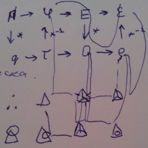
Diagram 5
Lines showing the Laplace operator (grad div A - rot rot A) for the composite idempotentIn regards to the convective term, because the term
))
is defined on the dual 3-cells, the term
))
is defined on the primal 2-cells, the term
))
has to be defined on the primal edges, and therefore
))
is defined on the dual 2-cell.
Since
is a 1-form, then

is a 1-form (in 3D), and therefore the wedge product is carried out between a 1-form and a 1-form, such that the outcome of this wedge product must be defined on the dual 2-cell.
Applying the exterior derivative operator to Eq. (4) (equivalent to taking the curl of the momentum equation Eq. (0a)), and considering the exterior derivative property dd = 0, the resulting governing equation is (expressions 6):
^{N+1} *^{-1}_F( \mu *d*^{-1}d*(d\mathbf{u}^\flat)) + (-1)^N d*^{-1}_F(\mathbf{u}^\flat \wedge*(d\mathbf{u}^\flat)) = 0)
,

^{N+1} ( \mu *d*^{-1}d*(d\mathbf{u}^\flat)) + (-1)^N d*_F d*^{-1}_F(\mathbf{u}^\flat \wedge*(d\mathbf{u}^\flat) = 0)
,